41 show data labels excel
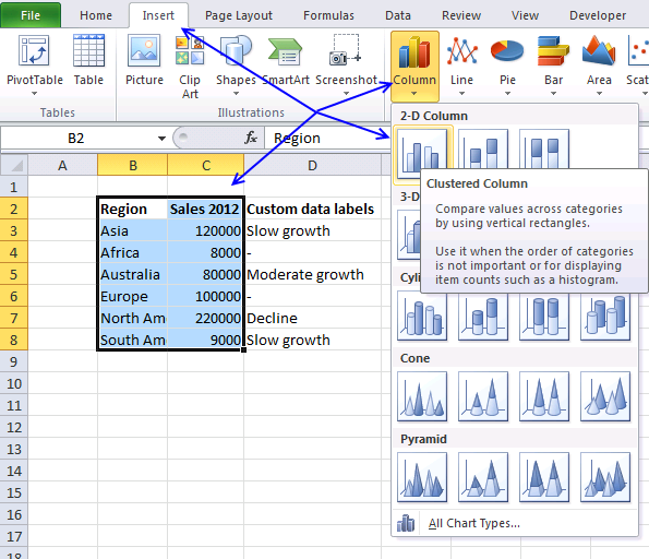
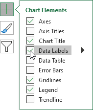
Excel tutorial: How to use data labels Generally, the easiest way to show data labels to use the chart elements menu. When you check the box, you'll see data labels appear in the chart. If you have more than one data series, you can select a series first, then turn on data labels for that series only. You can even select a single bar, and show just one data label. How to Add Data Labels in Excel - Excelchat | Excelchat After inserting a chart in Excel 2010 and earlier versions we need to do the followings to add data labels to the chart; Click inside the chart area to display the Chart Tools. Figure 2. Chart Tools. Click on Layout tab of the Chart Tools. In Labels group, click on Data Labels and select the position to add labels to the chart.
Custom data labels in a chart - Get Digital Help 21 Jan 2020 — Press with right mouse button on on any data series displayed in the chart. · Press with mouse on "Add Data Labels". · Press with mouse on Add ...
Show data labels excel
Custom Chart Data Labels In Excel With Formulas - How To Excel At Excel Follow the steps below to create the custom data labels. Select the chart label you want to change. In the formula-bar hit = (equals), select the cell reference containing your chart label's data. In this case, the first label is in cell E2. Finally, repeat for all your chart laebls. Add or remove data labels in a chart - support.microsoft.com In the upper right corner, next to the chart, click Add Chart Element > Data Labels. To change the location, click the arrow, and choose an option. If you want to show your data label inside a text bubble shape, click Data Callout. To make data labels easier to read, you can move them inside the data points or even outside of the chart. How to add data labels from different column in an Excel chart? Click any data label to select all data labels, and then click the specified data label to select it only in the chart. 3. Go to the formula bar, type =, select the corresponding cell in the different column, and press the Enter key. See screenshot: 4. Repeat the above 2 - 3 steps to add data labels from the different column for other data points.
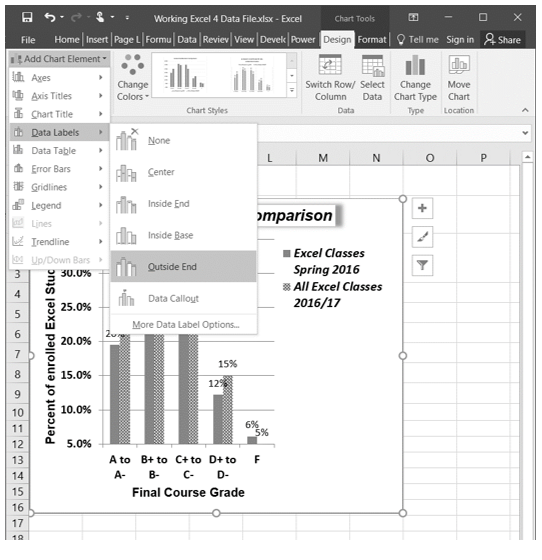
Show data labels excel. Find, label and highlight a certain data point in Excel scatter graph Select the Data Labels box and choose where to position the label. By default, Excel shows one numeric value for the label, y value in our case. To display both x and y values, right-click the label, click Format Data Labels…, select the X Value and Y value boxes, and set the Separator of your choosing: Label the data point by name, how to add data labels into Excel graphs You can download the corresponding Excel file to follow along with these steps: Right-click on a point and choose Add Data Label. You can choose any point to add a label—I'm strategically choosing the endpoint because that's where a label would best align with my design. Excel defaults to labeling the numeric value, as shown below. How to Change Excel Chart Data Labels to Custom Values? - Chandoo.org 05/05/2010 · Now, click on any data label. This will select “all” data labels. Now click once again. At this point excel will select only one data label. Go to Formula bar, press = and point to the cell where the data label for that chart data point is defined. Repeat the process for all other data labels, one after another. See the screencast. Enable or Disable Excel Data Labels at the click of a button - How To Step 1: Here is the sample data. Select and to go Insert tab > Charts group > Click column charts button > click 2D column chart. This will insert a new chart in the worksheet. Step 2: Having chart selected go to design tab > click add chart element button > hover over data labels > click outside end or whatever you feel fit.
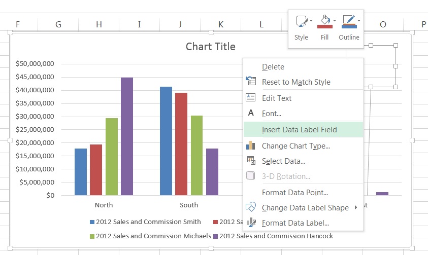
Format Data Labels in Excel- Instructions - TeachUcomp, Inc. To format data labels in Excel, choose the set of data labels to format. To do this, click the "Format" tab within the "Chart Tools" contextual tab in the Ribbon. Then select the data labels to format from the "Chart Elements" drop-down in the "Current Selection" button group. Then click the "Format Selection" button that ... How to hide zero data labels in chart in Excel? - ExtendOffice Tip: If you want to show the zero data labels, please go back to Format Data Labels dialog, and click Number> Custom, and select #,##0;-#,##0in the Typelist box. Data labels on small states using Maps - Microsoft Community Data labels on small states using Maps. Hello, I need some assistance using the Filled Maps chart type in Excel (note: this is NOT Power Maps). I have some data (see attachment below) that I've plotted on a map of the USA. Because the data only applied to 7 states I changed the "map area" (under Format Data Series-->Series Options) to show ... How To Create Labels In Excel - stgl.us Make Row Labels In Excel 2007 Freeze For Easier Reading from . Starting document near the bottom. Click a data label one time to select all data labels in a data series or two times to select just one data label that you want to delete, and then press delete. Click finish & merge in the finish group on the mailings tab.
Create Dynamic Chart Data Labels with Slicers - Excel Campus Step 3: Use the TEXT Function to Format the Labels. Typically a chart will display data labels based on the underlying source data for the chart. In Excel 2013 a new feature called “Value from Cells” was introduced. This feature allows us to specify the … DataLabels.ShowValue property (Excel) | Microsoft Docs This example enables the value to be shown for the data labels of the first series, on the first chart. This example assumes that a chart exists on the active worksheet. VB, Copy, Sub UseValue () ActiveSheet.ChartObjects (1).Activate ActiveChart.SeriesCollection (1) _ .DataLabels.ShowValue = True End Sub, Support and feedback, Display Data Label for first & last data points [SOLVED] Re: Display Data Label for first & last data points. My suggestion using a pivot table. However, data is in another layout in the "Data" sheet. When you add more data, simply refresh the pivot table (Data Sheet - Refresh). From the PivotTable Filter, select the Year you want to show on the graphs. Attached Files. Adding Data Labels to the Inside Ring of a Sunburst Chart : r/excel Once your problem is solved, reply to the answer (s) saying Solution Verified to close the thread. Follow the submission rules -- particularly 1 and 2. To fix the body, click edit. To fix your title, delete and re-post. Include your Excel version and all other relevant information. Failing to follow these steps may result in your post being ...
Quick Tip: Excel 2013 offers flexible data labels - TechRepublic
Excel charts: how to move data labels to legend @Matt_Fischer-Daly . You can't do that, but you can show a data table below the chart instead of data labels: Click anywhere on the chart. On the Design tab of the ribbon (under Chart Tools), in the Chart Layouts group, click Add Chart Element > Data Table > With Legend Keys (or No Legend Keys if you prefer)
4.2 Formatting Charts – Beginning Excel
Displaying Large Numbers in K (thousands) or M (millions) in Excel How To Display Numbers in Millions in Excel, Right-Click any number you want to convert. Go to Format Cells. In the pop-up window, move to Custom formatting. If you want to show the numbers in Millions, simply change the format from General to 0,,"M" . The figures will now be 23M.

Enable or Disable Excel Data Labels at the click of a button - How To - PakAccountants.com
Change the format of data labels in a chart To get there, after adding your data labels, select the data label to format, and then click Chart Elements > Data Labels > More Options. To go to the appropriate area, click one of the four icons ( Fill & Line , Effects , Size & Properties ( Layout & Properties in Outlook or Word), or Label Options ) shown here.

410 How to display percentage labels in pie chart in Excel 2016 - YouTube
How To Show Or Hide Data Labels On MS Excel? 22 Dec 2019 — Select the chart on your MS Excel worksheet, A plus sign will appear at the top right corner of the table. · Now, you need to point to Data ...

MS Excel 2010 / How to display data labels on the chart - YouTube
to display top 5 data labels on graph [SOLVED] Re: to display top 5 data labels on graph. Also, I noticed your sum column ("total") is returning errors. I don't see why you would want to do this, and in fact I'm not even sure why excel wanted to do this to begin with. if you run C3+D3 when those cells are empty, excel should return 0. So I got rid of the error, and that way, you can use the ...
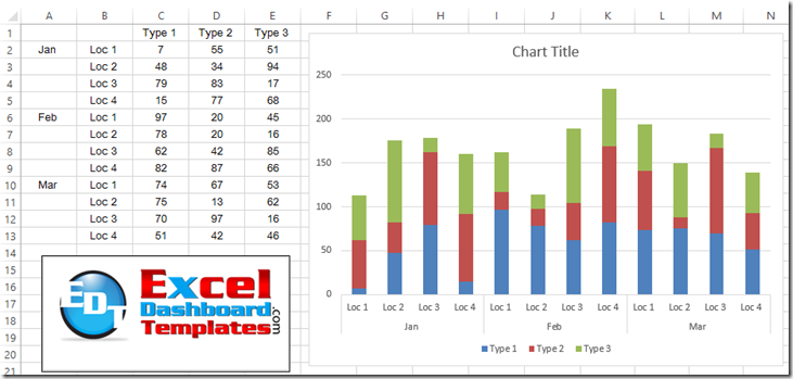
How-to Graph Three Sets of Data Criteria in an Excel Clustered Column Chart - Excel Dashboard ...
How to add data labels in excel to graph or chart (Step-by-Step) 1. Select a data series or a graph. After picking the series, click the data point you want to label. 2. Click Add Chart Element Chart Elements button > Data Labels in the upper right corner, close to the chart. 3. Click the arrow and select an option to modify the location. 4.

How to Add Data Labels in Excel - Excelchat | Excelchat
How to use data labels in a chart - YouTube Excel charts have a flexible system to display values called "data labels". Data labels are a classic example a "simple" Excel feature with a huge range of o...

EXCEL: SETTING PIVOT TABLE DEFAULTS - Strategic Finance
How to Use Cell Values for Excel Chart Labels - How-To Geek 12/03/2020 · Make your chart labels in Microsoft Excel dynamic by linking them to cell values. When the data changes, the chart labels automatically update. In this article, we explore how to make both your chart title and the chart data labels dynamic. We have the sample data below with product sales and the difference in last month’s sales.

How to format data labels in excel charts and data elements - YouTube
Text Labels on a Horizontal Bar Chart in Excel - Peltier Tech 21/12/2010 · In this tutorial I’ll show how to use a combination bar-column chart, in which the bars show the survey results and the columns provide the text labels for the horizontal axis. The steps are essentially the same in Excel 2007 and in Excel 2003. I’ll show the charts from Excel 2007, and the different dialogs for both where applicable.

How to sort data with Microsoft Excel 2016 - MATC Information Technology Programs: Degrees ...
Edit titles or data labels in a chart - Microsoft Support On a chart, do one of the following: To reposition all data labels for an entire data series, click a data label once to select the data series. · On the Layout ...

30 Label The Excel Window - Labels Design Ideas 2020
How to Add Total Data Labels to the Excel Stacked Bar Chart 03/04/2013 · Step 4: Right click your new line chart and select “Add Data Labels” Step 5: Right click your new data labels and format them so that their label position is “Above”; also make the labels bold and increase the font size. Step 6: Right click the line, select “Format Data Series”; in the Line Color menu, select “No line”

Chapter 3 Excel 2007/2010 Charts
How to show data label in "percentage" instead of - Microsoft Community Select Format Data Labels, Select Number in the left column, Select Percentage in the popup options, In the Format code field set the number of decimal places required and click Add. (Or if the table data in in percentage format then you can select Link to source.) Click OK, Regards, OssieMac, Report abuse, 8 people found this reply helpful, ·,
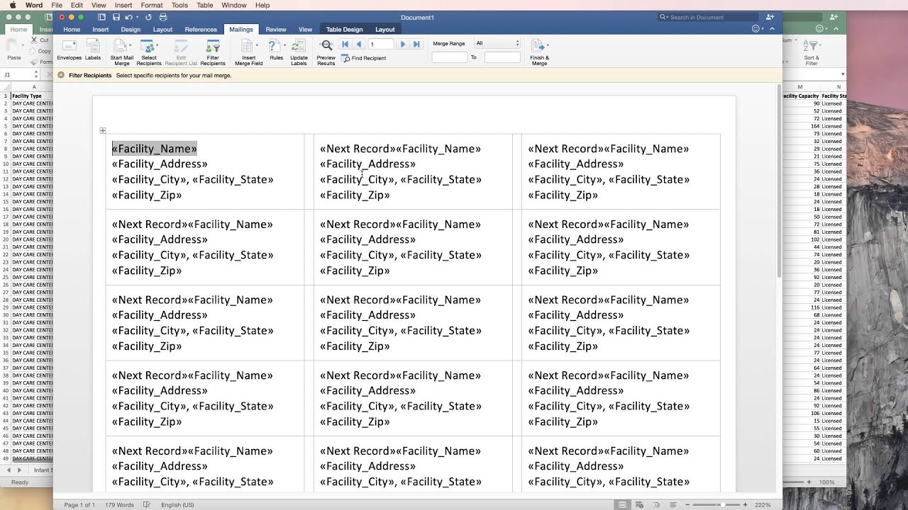
How To Create Mailing Labels - Mail Merge Using Excel and Word from Office 365 - YouTube
Hiding data labels for some, not all values in a series Here's a good challenge for you. I can't figure it out, and I believe it's a limitation of Excel. I have a bar graph with several data series. I know how to show the data labels for every data point in a given series. But I'm looking to show the data label for only some data points in a given series -- i.e. non-zero valued data points.

Excel 2013 Tutorial Formatting Data Labels Microsoft Training Lesson 28.6 - YouTube
How to show percentage in pie chart in Excel? - ExtendOffice Show percentage in pie chart in Excel. Please do as follows to create a pie chart and show percentage in the pie slices. 1. Select the data you will create a pie chart based on, click Insert > Insert Pie or Doughnut Chart > Pie. See screenshot: 2. Then a pie chart is created. Right click the pie chart and select Add Data Labels from the context ...
Custom data labels in a chart | Get Digital Help - Microsoft Excel resource
Prevent Overlapping Data Labels in Excel Charts - Peltier Tech 24/05/2021 · make the labels show the Y value and series name of the labeled series.Position = xlLabelPositionLeft.Position = xlLabelPositionRight ... An internet search of “excel vba overlap data labels” will find you many attempts to solve the problem, with various levels of success. I’ve implemented a few different approaches in various projects ...

Excel Treemap - Beat Excel!
Add a DATA LABEL to ONE POINT on a chart in Excel All the data points will be highlighted. Click again on the single point that you want to add a data label to. Right-click and select ' Add data label '. This is the key step! Right-click again on the data point itself (not the label) and select ' Format data label '. You can now configure the label as required — select the content of ...
Create Charts in Excel - Easy Excel Tutorial
How to Add Data Labels to an Excel 2010 Chart - dummies On the Chart Tools Layout tab, click Data Labels→More Data Label Options. The Format Data Labels dialog box appears. You can use the options on the Label Options, Number, Fill, Border Color, Border Styles, Shadow, Glow and Soft Edges, 3-D Format, and Alignment tabs to customize the appearance and position of the data labels.
SQL Workbench/J User's Manual SQLWorkbench
Adding Colored Regions to Excel Charts - Duke Libraries Center for Data ... 12/11/2012 · Right-click on the individual data series to change the colors, line widths, etc. Use the formatting options or the Chart tools on the Excel ribbon to change the font of any text, adjust the grid lines, add labels and titles, etc. The data series names in the legend can be adjusted by using the “Select Data…” option and typing in custom ...
Post a Comment for "41 show data labels excel"