42 how to add two data labels in excel pie chart
How to Use Cell Values for Excel Chart Labels Select the chart, choose the "Chart Elements" option, click the "Data Labels" arrow, and then "More Options." Uncheck the "Value" box and check the "Value From Cells" box. Select cells C2:C6 to use for the data label range and then click the "OK" button. The values from these cells are now used for the chart data labels. How to Combine or Group Pie Charts in Microsoft Excel For example, the pie chart below shows the answers of people to a question. This is fine, but it can be complicated if you have multiple Pie charts. Pie charts can only show one series of values. So if you have multiple series, and you want to present data with pie charts, you need multiple pie charts.
Create two data labels in pie chart? | MrExcel Message Board Aug 30, 2018 — There are 50 pie charts and I don't want to manually adjust each one. Suggestions? Excel Facts.3 answers · 0 votes: Hi, Sorry but maybe I didn’t make that very clear. I intended that you simply put the icon/image ...
How to add two data labels in excel pie chart
Excel charts: add title, customize chart axis, legend and data labels ... Click the Chart Elements button, and select the Data Labels option. For example, this is how we can add labels to one of the data series in our Excel chart: For specific chart types, such as pie chart, you can also choose the labels location. For this, click the arrow next to Data Labels, and choose the option you want. › charts › axis-labelsHow to add Axis Labels (X & Y) in Excel & Google Sheets How to Add Axis Labels (X&Y) in Excel. Graphs and charts in Excel are a great way to visualize a dataset in a way that is easy to understand. The user should be able to understand every aspect about what the visualization is trying to show right away. As a result, including labels to the X and Y axis is essential so that the user can see what ... Add or remove data labels in a chart - support.microsoft.com Click the data series or chart. To label one data point, after clicking the series, click that data point. In the upper right corner, next to the chart, click Add Chart Element > Data Labels. To change the location, click the arrow, and choose an option. If you want to show your data label inside a text bubble shape, click Data Callout.
How to add two data labels in excel pie chart. Pie of Pie Chart in Excel - Inserting, Customizing, Formatting To add the data labels:- Select the chart and click on + icon at the top right corner of chart. Mark the check box containing data labels. Formatting Data Labels Consequently, this is going to insert default data labels on the chart. How to Map Data in Excel (2 Easy Methods) - ExcelDemy First of all, select the range of the dataset as shown below. Next, go to the Insert tab from your ribbon. Then, select Maps from the Charts group. Now, select the Filled Map icon from the drop-down list. As a result, you will get the following map chart of countries. Add a DATA LABEL to ONE POINT on a chart in Excel Method — add one data label to a chart line Steps shown in the video above: Click on the chart line to add the data point to. All the data points will be highlighted. Click again on the single point that you want to add a data label to. Right-click and select ' Add data label ' This is the key step! › charts › add-data-pointAdd Data Points to Existing Chart – Excel & Google Sheets Start with your Graph. Similar to Excel, create a line graph based on the first two columns (Months & Items Sold) Right click on graph; Select Data Range; 3. Select Add Series. 4.
How to add data labels from different column in an Excel chart? Right click the data series in the chart, and select Add Data Labels > Add Data Labels from the context menu to add data labels. 2. Click any data label to select all data labels, and then click the specified data label to select it only in the chart. 3. How to fix wrapped data labels in a pie chart - Sage Intelligence 1. Right click on the data label and select Format Data Labels 2. Select Text Options > Text Box > and un-select Wrap text in shape. 3. The data labels resize to fit all the text on one line. 4. Alternatively, by double-clicking a data label, the handles can be used to resize the label to wrap words as desired. How To Add Data Labels In Excel - lakesidebaptistchurch.info First add data labels to the chart (layout ribbon > data labels) define the new data label values in a bunch of cells, like this: Open your desired excel file. Source: superuser.com. To format data labels, select your chart, and then in the chart design tab, click add chart element > data labels > more data label options. Adding Data Labels to Your Chart (Microsoft Excel) To add data labels in Excel 2013 or Excel 2016, follow these steps: Activate the chart by clicking on it, if necessary. Make sure the Design tab of the ribbon is displayed. (This will appear when the chart is selected.) Click the Add Chart Element drop-down list. Select the Data Labels tool.
Creating Pie Chart and Adding/Formatting Data Labels (Excel) Creating Pie Chart and Adding/Formatting Data Labels (Excel) Creating Pie Chart and Adding/Formatting Data Labels (Excel) › data-series-data-points-dataUnderstanding Excel Chart Data Series, Data Points, and Data ... Sep 19, 2020 · Add Emphasis With a Combo Chart . Another option for emphasizing different types of information in a chart is to display two or more chart types in a single chart, such as a column chart and a line graph. You could use this approach when the graphed values vary widely or when graphing different types of data. How to Create and Format a Pie Chart in Excel - Lifewire To add data labels to a pie chart: Select the plot area of the pie chart. Right-click the chart. Select Add Data Labels . Select Add Data Labels. In this example, the sales for each cookie is added to the slices of the pie chart. Change Colors › pie-chart-examplesPie Chart Examples | Types of Pie Charts in Excel ... - EDUCBA Now our task is to add the Data series to the PIE chart divisions. Click on the PIE chart so that the chart will get a highlight, as shown below. Right-click and choose the “Add Data Labels “option for additional drop-down options.
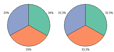
Pie Chart Rounding in Excel - Peltier Tech Blog
Pivot Chart Data Label Help Needed - Microsoft Community Open the Excel file with Pivot Chart and enabled with Data Labels> Click on the Labels displayed in the Chart> Right-click> Click Format Data Labels> Label Options> Number> In the Category, select the format as per your requirement. Here is the reference article: Change the format of data labels in a chart.
Post a Comment for "42 how to add two data labels in excel pie chart"